
The ARRT CT exam assesses entry-level computed tomography knowledge against content specifications effective September 1, 2026: 165 scored questions plus 30 unscored pilot items in 195 minutes. Procedures carries the largest share (71 questions), followed by Image Production (52), then Patient Care and Safety (21 each). Build your study order around those weights and your own weak areas, work from the official content outline rather than secondhand summaries, and confirm eligibility details in the current postprimary handbook before you apply.
What the ARRT CT credential is
The credential is the ARRT Registered Technologist (R.T.) credential in Computed Tomography, earned through the postprimary pathway. The exam tests the knowledge and cognitive skills behind entry-level CT practice, and the current content specifications took effect September 1, 2026.
Computed Tomography is one of ARRT's postprimary credentials: you pursue it after establishing eligibility in a supporting discipline, not as a first credential. If you have seen it written as "CT (AC)", note that AC is not part of the official credential name; ARRT lists the discipline simply as Computed Tomography.
ARRT built the exam from a practice analysis of what entry-level CT technologists typically do, and the published purpose is to assess whether candidates have the knowledge and cognitive skills underlying that entry-level work. The companion Task Inventory for Computed Tomography is on ARRT's website, and every content category in the outline links to tasks on that inventory.
Version matters for your preparation. The current Examination Content Specifications for Computed Tomography were board approved in July 2025 and take effect on September 1, 2026, replacing the prior edition. Study from the document dated on or after that implementation date, and check ARRT's content specifications page for any newer release.
Official sources: ARRT Computed Tomography Content Specifications effective September 1, 2026 — Content category table and content outline; Examination Content Specifications - ARRT (arrt.org) — Credential list including Computed Tomography; ARRT Postprimary Eligibility Pathway Handbook (2026) — Eligibility, application, exam format, and security sections
Eligibility through the postprimary pathway
You may qualify if you already hold a supporting ARRT credential, hold a supporting credential from another ARRT-recognized organization, or have your program director's permission to log requirements while finishing your program. Every candidate must satisfy education, ethics, and examination requirements.
ARRT frames its credential as education plus ethics plus examination. For CT, the education requirement combines structured education and clinical experience within your eligibility period, and the ethics requirement involves agreeing to ARRT's Standards of Ethics.
You may be eligible to pursue a postprimary credential if you have done at least one of the following: earned a supporting ARRT credential through the primary pathway, earned a supporting credential from another ARRT-recognized organization, or received your program director's permission to begin logging the clinical experience and structured education requirements while completing your educational program.
Two policies shape your timeline. First, you must pass within your eligibility period, and the re-examination policy allows three attempts in three years. Second, ARRT updates its handbooks yearly and states that you should review the most current handbook before you apply, because policies can change during your eligibility period.
The retrieved handbook passages do not include the specific structured-education hour counts or clinical-experience volumes for CT. Before you apply, read the education requirements section of the current postprimary eligibility pathway handbook on arrt.org and confirm the exact numbers that apply to you.
Official sources: ARRT Postprimary Eligibility Pathway Handbook (2026) — Eligibility, application, exam format, and security sections
Explore in 3D: Heart chambers and great vessels
A four-chambered heart viewed from the front. The right ventricle supplies the pulmonary circulation via the pulmonary trunk; the left ventricle supplies the systemic circulation via the ascending aorta. This model shows external chamber surfaces and the visible great vessels only — no internal valves or conduction system.
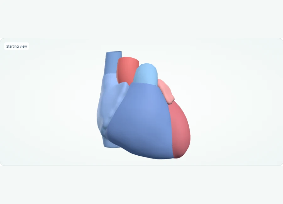
Rotate, isolate structures, and test your recall.
Choose Front and compare the four chambers. The right ventricle forms most of the anterior surface; the left ventricle contributes to the apex.
Select and isolate each chamber in turn, then use Show all to restore its relationship to the surrounding structures.
Select the pulmonary trunk and ascending aorta in turn. Name the circulation supplied by each, then use Test recall to practise identifying the listed structures.
Practice exercise
Which ventricle supplies the pulmonary trunk, and which supplies the ascending aorta?
Show answer
The right ventricle; it serves the pulmonary circulation.
On the front view, the right ventricle is the anterior-most chamber, and its outflow tract continues as the pulmonary trunk carrying blood to the lungs. The left ventricle instead empties into the ascending aorta for the systemic circulation.
- The right ventricle pumps blood into the pulmonary trunk toward the lungs; the left ventricle pumps into the ascending aorta to the body.
- The superior vena cava returns blood to the right atrium from above the heart.
- The two atria sit superior to the two ventricles; atria receive blood, ventricles eject it.
Exam format and question counts
The CT exam has 165 scored questions plus 30 unscored pilot questions, with 195 minutes of test time inside a 3 hour 35 minute appointment. Most questions are multiple choice with one best answer, presented in random order.
The content specifications fix the question distribution: 165 scored questions, plus an additional 30 unscored pilot questions used to evaluate potential questions for future exams. Pilot questions are not identified during the exam, and your answers to them do not affect your score.
Format varies beyond plain multiple choice. Some questions ask you to select multiple answers from a list, sort options into order with your mouse, click a region of an image on screen, or answer after watching a short video clip. Questions appear in random order, which ARRT describes as a way to let you show you can access the material outside a specific context.
A few administrative rules are worth memorizing. You must accept the nondisclosure agreement within two minutes of it appearing. Bring two valid forms of acceptable ID, arrive 30 minutes early, and leave phones and other belongings outside the test area. Arriving without proper ID means you cannot test, you forfeit the application fee, and you must reapply and pay again.
Official sources: ARRT Computed Tomography Content Specifications effective September 1, 2026 — Content category table and content outline; ARRT Postprimary Eligibility Pathway Handbook (2026) — Eligibility, application, exam format, and security sections
Content categories and question weights
Procedures carries 71 scored questions, Image Production 52, Patient Care 21, and Safety 21. Those official weights are the most defensible starting point for deciding how to divide your study time.
The table below reproduces the official category counts from the 2026 content specifications. Each category also has subcategories; for example, Image Production splits into Image Formation (30 questions) and Image Evaluation and Archiving (22), and Procedures splits into Head, Spine, and Musculoskeletal (25), Neck and Chest (22), and Abdomen and Pelvis (24).
One content note from ARRT itself: SI units are the primary units of radiation measurement used on the CT examination. When you practice dose calculations, work in milligray and related SI-derived units rather than traditional units.
Weights describe the exam, not your personal gaps. A category worth few questions can still deserve extra time if it is where you are weakest; the arithmetic below simply sets a floor for the large categories.
Practice exercise
Using the official counts in the table (Patient Care 21, Safety 21, Image Production 52, Procedures 71, total 165), what percentage of the scored questions comes from Procedures? If you have 40 total hours to study and divide time strictly in proportion to these weights, how many hours does Procedures receive?
Show answer
Procedures accounts for 71 ÷ 165 ≈ 43% of scored questions. Strictly proportional allocation gives 0.43 × 40 ≈ 17 hours for Procedures, about 12.6 hours for Image Production (52 ÷ 165 ≈ 32%), and about 5.1 hours each for Patient Care and Safety (21 ÷ 165 ≈ 13% each).
This is pure arithmetic on the officially published question counts, so the shares are exact rather than estimated. The allocation is illustrative: proportional time is a sensible floor for the large categories, but you should shift hours toward categories where your self-assessment and practice results show weaknesses, and any study schedule is editorial advice, not an ARRT requirement.
| Content category | Scored questions |
|---|---|
| Patient Care (Patient Interactions and Management) | 21 |
| Safety (Radiation Safety and Dose) | 21 |
| Image Production (Image Formation 30; Image Evaluation and Archiving 22) | 52 |
| Procedures (Head, Spine, and Musculoskeletal 25; Neck and Chest 22; Abdomen and Pelvis 24) | 71 |
| Total scored | 165 |
Official sources: ARRT Computed Tomography Content Specifications effective September 1, 2026 — Content category table and content outline
Preparation priorities by category
Work from the official outline, not a summary. Patient Care covers assessment, contrast media, venipuncture, and reaction recognition; Safety covers physics, dose metrics, and protection; Image Production covers parameters, reconstruction, and artifacts; Procedures covers cross-sectional anatomy and protocol factors study by study.
Patient Care (21 questions). The outline lists patient assessment and preparation, scheduling and screening, interpersonal communication, lab values such as renal function markers, consent types, ergonomics and transfer techniques, patient monitoring, contrast media types and properties with special considerations such as pregnancy and dialysis, noncontrast medications, venipuncture, injection and scanning techniques, contrast reaction recognition and classification, and postprocedure care. Use this list to audit your notes; anything not on it is background, not tested content.
Safety (21 questions). Expect radiation physics (x-ray production, target interactions, photon interactions), radiation protection levers (kVp, mAs, pitch, collimation, filtration, gating, dose modulation), shielding, patient considerations, dose measurements, and personnel protection. The dose metrics named in the outline include absorbed dose, effective dose, CT dose index (CTDI), and dose-length product (DLP). Remember that SI units are primary on this exam.
Image Production (52 questions). This category spans CT unit components, imaging parameters, data acquisition methods, image reconstruction, postprocessing, image display and quality, artifact recognition and reduction, and informatics such as PACS and DICOM. The artifact list is specific: beam hardening, partial volume averaging, motion, metallic, edge gradient, out-of-field positioning, and equipment artifacts such as rings and streaks. Learning that named list is a straightforward, high-value task.
Procedures (71 questions). Questions on each study type can address anatomy and physiology with cross-sectional anatomy and pathological recognition, factors such as imaging planes, protocol considerations, and patient considerations, contrast media with indications and scan or prep delays, and additional procedures such as CTA, biopsy, and trauma. The named study list runs from head, spine, and musculoskeletal studies through neck and chest studies including cardiac gating and lung screening, to abdomen and pelvis studies including multiphase liver, pancreas, adrenals, kidneys, and colonography. Review sectional anatomy region by region against this list.
A note on scope: these are preparation priorities drawn from the official outline's topic lists. The outline identifies what is tested; it does not replace a supervised clinical education or a protocol manual, and paper preparation alone cannot establish practical competence.
Practice exercise
Assume a single abdominal series is acquired with a volume CT dose index (CTDIvol) of 8 mGy over a scan length of 30 cm, and assume that the dose-length product (DLP) for the series equals CTDIvol multiplied by scan length. What is the DLP, and why do the units combine the way they do?
Show answer
DLP = 8 mGy × 30 cm = 240 mGy·cm. The units combine because mGy multiplied by cm gives mGy·cm, exactly the unit ARRT's outline lists for dose-length product.
The multiplication rule is stated as an assumption in the prompt, so the only work required is unit arithmetic, which checks independently: mGy × cm = mGy·cm. Practicing the unit structure is useful because the exam uses SI-derived dose units, and the outline lists CTDI in mGy and DLP in mGy·cm as distinct dose measurements. Real protocol values and any dose limits or notifications come from your facility's equipment and policies, not from this calculation.
Official sources: ARRT Computed Tomography Content Specifications effective September 1, 2026 — Content category table and content outline
Test-day checklist and pitfalls to avoid
Confirm your ID documents, appointment logistics, and the nondisclosure timing before exam day. On the exam itself, flag hard questions and return to them, and remember that pilot questions do not count.
The night before, verify two things: that you have two valid, signed forms of acceptable ID whose names match your ARRT file, and that you know your appointment time. Plan to arrive 30 minutes early, and cancel or reschedule properly if you cannot attend, because missing your appointment or failing to cancel correctly closes your window and forfeits your application fee.
At the test center, accept the nondisclosure agreement within two minutes of it appearing. During the exam, flag difficult questions and return to them if time allows, and do not agonize over possible pilot questions; they are unmarked and unscored.
One rule protects your credential long after test day: never disclose exam content using language substantially similar to ARRT's questions or answer options, to or from anyone, including students, educators, and exam-preparation providers. Violations can lead to sanctions, including ineligibility or revocation. Use preparation materials that teach the published outline instead of recalled questions.
- Bring two valid forms of acceptable ID, signed, with names matching your ARRT file.
- Arrive 30 minutes before your appointment.
- Accept the nondisclosure agreement within two minutes of accessing it.
- Flag difficult questions and return to them if time allows.
- Ignore pilot-question guesses; they do not affect your score.
- Never share or seek exam content in language similar to real questions or answer options.
Official sources: ARRT Postprimary Eligibility Pathway Handbook (2026) — Eligibility, application, exam format, and security sections
Official sources
Facts checked against ARRT documents: